Chiller Plant Optimization

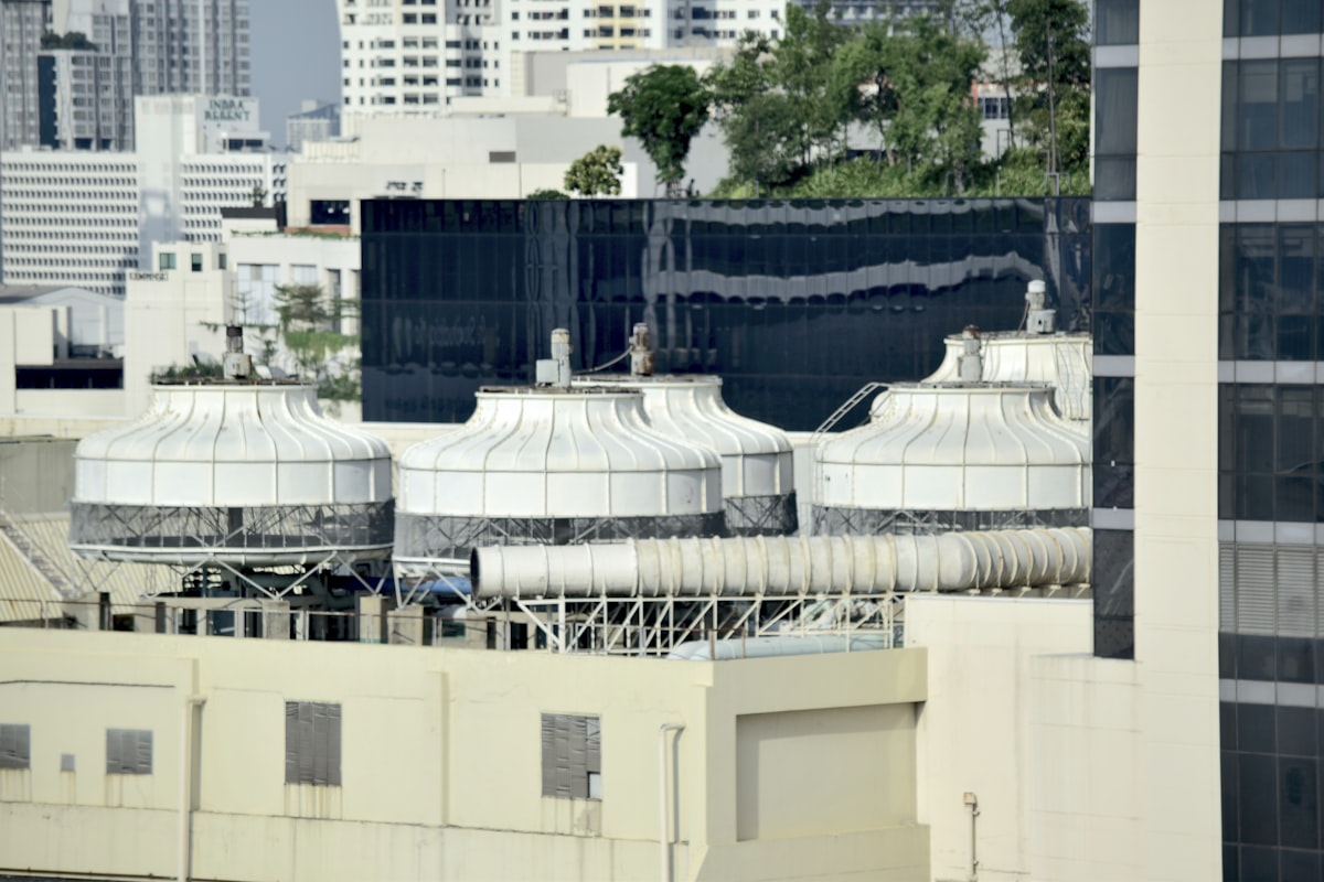
Photo by Nopparuj Lamaikul on Unsplash.

A chiller's own controller already reports the four numbers that matter most for running the plant well: how closely the condenser and evaporator approach their theoretical temperature limits, how much superheat sits at the compressor suction, how many amps the compressor draws for a given load, and how often the machine starts and stops. Chiller plant optimization is the practice of reading those numbers with two questions running at once. Is anything degrading. Is anything costing more to run than it should. Most published material treats those as two disciplines with two sets of reports. They are the same readings.

Nearly every commercial chiller already trends this data somewhere, either in the unit’s own controller log or in the building automation system under point names like cond appr temp and comp amps A. The gap is rarely instrumentation. It is that nobody reads a trend with both questions in mind, so a reading that would flag a maintenance finding this month and a cost finding next quarter gets read for neither.

The signals a chiller already gives you

Condenser approach temperature is the gap between the refrigerant’s condensing temperature and the temperature of whatever is rejecting that heat: condenser water on a water-cooled machine, outdoor air on an air-cooled one. A clean condenser typically holds a tight approach. Let that gap widen and the machine is pushing heat across a layer of thermal resistance nobody designed in, usually scale or biofilm on the tubes, or a fouled coil.

Evaporator approach temperature is the same idea on the chilled-water side: the gap between the refrigerant’s evaporating temperature and the leaving chilled-water temperature. It widens for related reasons, tube fouling, low refrigerant charge, or reduced flow, but on the load side of the machine rather than the heat-rejection side.

Superheat is how far the refrigerant’s temperature sits above its saturation point at the compressor suction, and it is usually the earliest number to move when metering or charge is off. Superheat running low risks liquid refrigerant reaching the compressor. Superheat running high usually means the evaporator is starved, and the compressor is working harder to deliver the same cooling.

Compressor amps, read against chilled-water flow and delta-T where the controller reports tonnage, is the closest thing to a direct efficiency reading most plants have without a dedicated power meter. Amps climbing for a load that has not changed is degradation showing up in the present tense, not a forecast.

Cycle counts and starts-per-hour measure something different: not thermal performance but mechanical wear and control stability. A compressor cycling a dozen times an hour never settles into steady operation between starts, which is harder on the machine and less efficient than one long, steady run at a lower load.

Why the same reading is two findings

Each of those five readings answers a maintenance question and a cost question with the same value, because heat transfer and electrical draw are mechanically linked inside a chiller. A wider approach temperature means the refrigerant has to run at a more extreme pressure to move the same heat across a fouled surface, and pressure differential is what the compressor works against. Every degree of avoidable approach is a degree the compressor did not need to lift or drop, and that shows up as amps.

Superheat and cycle counts carry the same double meaning from a different angle. Starved superheat means the compressor works longer for less cooling per cycle. Short-cycling means the machine spends a disproportionate share of its runtime in the least efficient part of its operating curve, the ramp between start and steady state, rather than in the flat, efficient middle. Neither of those is a separate energy problem sitting next to a separate mechanical one. They are the same fault, described twice.

This is the part most condition monitoring writing skips, because it is written for rotating machinery in general and a chiller is a specific thermodynamic exception. A bearing wearing out on a fan does not usually change the fan’s electrical draw much until it is close to failure. A chiller losing heat-transfer efficiency changes its electrical draw immediately and continuously, in rough proportion to how far it has drifted. That is what makes chiller plant optimization worth treating as its own discipline rather than a subset of general condition monitoring.

A worked example: short-cycling that isn't a broken compressor

Take a plant with two chillers on a lead-lag staging sequence, sized so one machine covers the building’s normal load and the second only comes on during peak demand. The BMS trend shows the lag chiller cycling on and off every fifteen to twenty minutes through a mild afternoon, well short of its rated minimum run time. The obvious read is a failing compressor or a stuck contactor.

Usually it isn’t. The more common cause is a staging deadband set too narrow for the load swing the building actually produces, so a small dip in chilled-water demand drops the plant below the lag chiller’s cut-out point almost as soon as it cuts in. A second common cause is a return-temperature sensor that has drifted a degree or two, feeding the staging logic a signal that no longer matches reality. A third is a lead-lag rotation schedule that swaps which chiller is primary on a fixed calendar rather than on runtime, so a machine that should be resting gets called into a load band it was never staged for.

All three are control problems, not mechanical failures, and all three are visible in the readings above before a technician opens a panel. Compressor amps show short runs that never reach steady draw. Cycle counts climb against that unit’s own history for the season. Approach temperatures on the lag chiller barely move, because the machine never runs long enough to develop a clean baseline, which is itself worth flagging. Chasing this as a hardware fault means a service call that finds nothing wrong with the compressor. Reading it as a staging problem means adjusting a deadband or correcting a sensor offset, at a fraction of the cost and downtime.

What's already trending, and what's worth adding

Most of what this piece covers is not a hardware project. Chiller controllers from every major manufacturer already log approach temperatures, superheat, amps and cycle counts internally, whether or not that data ever leaves the unit. Where a BMS is integrated with the chiller over BACnet or Modbus, those same points are usually already mapped and trending, just unread. The typical starting gap is not sensors. It is nobody having built the habit of pulling the trend and asking both questions of it.

The exceptions worth flagging: many plants don’t meter chilled-water flow directly, which means a true kW-per-ton figure has to be estimated from amps and load rather than measured, and standalone chillers without a networked controller may only expose alarm points rather than continuous trend data. Both are solvable, but they are the minority case, not the starting point. Start with what the controller and BMS already report before specifying anything new.

From a wall of trend charts to a ranked queue

Reading five signals across every chiller in a plant, across every season, by eye does not scale past one or two machines. What changes the economics is a system that reads the same points continuously, learns what each machine’s own normal looks like across a full heating and cooling season, and surfaces a drift with a plain-language reason rather than another chart to interpret. That is the detection engine FrostLogic Explore runs on top of existing BMS and chiller controller data: it reads the points already there, ranks what is drifting furthest from its own baseline, and returns a queue ordered by what is worth attention first, rather than a dashboard that assumes someone has time to go looking.

A rising approach temperature or a climbing amp draw is also exactly the kind of signal that feeds a building’s broader energy management software, since a degrading chiller is one of the larger swings a facility’s utility bill will see. Chiller-level detection is one input into that wider picture, not a replacement for it.

The staging-sequence reasoning in the worked example above is specific to comfort-cooling chillers in buildings. For the same kind of thinking applied to industrial process equipment, we’ve covered predictive maintenance in manufacturing separately.

FAQ

What is chiller plant optimization?
Reading a chiller’s own approach temperatures, superheat, compressor amps and cycle counts as both a maintenance signal and an energy-cost signal, rather than tracking them in separate reports. The two questions, is something degrading and is something costing more to run, are answered by the same trend.

How is chiller plant optimization different from condition monitoring?
Condition monitoring is the broader practice across every asset in a plant room, pumps, fans, air handling units and chillers alike, asking whether an asset is degrading. Chiller plant optimization is the chiller-specific version of that question, extended to explicitly connect the same readings to running cost rather than health alone. We’ve covered condition monitoring for buildings generally elsewhere; this page is the deeper, chiller-specific layer underneath it.

Does chiller plant optimization replace a CMMS?
No. Explore is a decision layer, not a CMMS. It does not manage work orders, hold PM schedules, track spare parts or dispatch technicians. It identifies which chiller signal is drifting and why, so the resulting work still gets planned and tracked in whatever CMMS a team already runs.

Is chiller plant optimization the same as energy management?
Related but narrower. Energy management software looks at a building’s or portfolio’s total consumption and cost across every system. Chiller plant optimization is one input into that picture, focused specifically on what a chiller’s own control signals reveal about its condition and efficiency.

What data do I need to start reading chiller signals this way?
Usually nothing beyond what the chiller controller and BMS already trend. Approach temperatures, superheat, amps and cycle counts are standard controller outputs on most commercial machines. The common gap is a chilled-water flow meter for a true kW-per-ton reading, worth adding once the existing signals show where to look.

What usually causes chiller short-cycling?
More often a staging or control-sequence fault than a failing compressor: a deadband set too tight for the load, a drifted sensor feeding the staging logic bad data, or a lead-lag rotation running on a fixed schedule rather than on runtime. All three show up in compressor amps and cycle counts before a technician needs to open a panel.

How often should condenser approach temperature be checked?
Continuously is better than periodically, since the value that matters is the trend against the machine’s own baseline rather than a single reading. Where trending isn’t automated, a monthly manual check against the manufacturer’s clean-condenser approach spec is the minimum useful cadence.